How to Draw Chart Bar Google Docs
Look, while they're certainly not the easiest way to consume information, most companies are still using spreadsheets in order to pull a lot of different data into one place.
That's the strength of a Spreadsheet–collating a lot of information in one place.
And while there's a lot of functionality within a tool like Google Sheets to categorize and manipulate the data, it's not the best tool to present performance data to others.
That's why most people who put together Spreadsheets also look for ways to visualize the data inside of it. This way, it's more accessible to others, whether that's members of your own team, your bosses, or even board of directors.
Here's how to easily create a bar graph (or other visualizations) using your performance data in Google Sheets.
- How to Create a Bar Graph in Google Sheets
- How to Label a Bar Graph in Google Sheets
- How to Change a Visualization in Google Sheets
- How to Add Error Bars in Google Sheets
- How to Integrate Google Sheets with Databox

How to Create A Bar Graph in Google Sheets
For the full written tutorial, continue reading. Prefer step-by-step video tutorial? View the 4-minute clip right here…
Now, for the written tutorial…You can create a bar graph in Google Sheets in 3 simple steps:
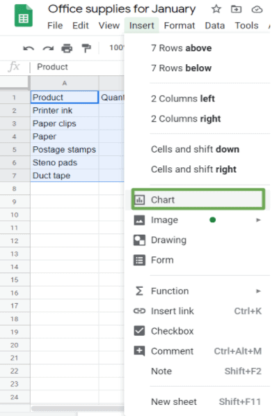
- Highlight the cells containing the data you'd like to visualize
- Click the 'Chart' icon in the Google Sheets toolbar
- Customize and/or change the visualization type in the chart editor
First, you'll want to highlight the specific cells you're looking to visualize.
In the example below, I'm going to highlight revenue from our fictional online book shop from Q1.
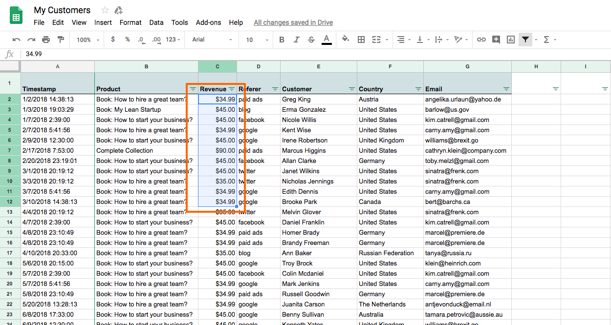
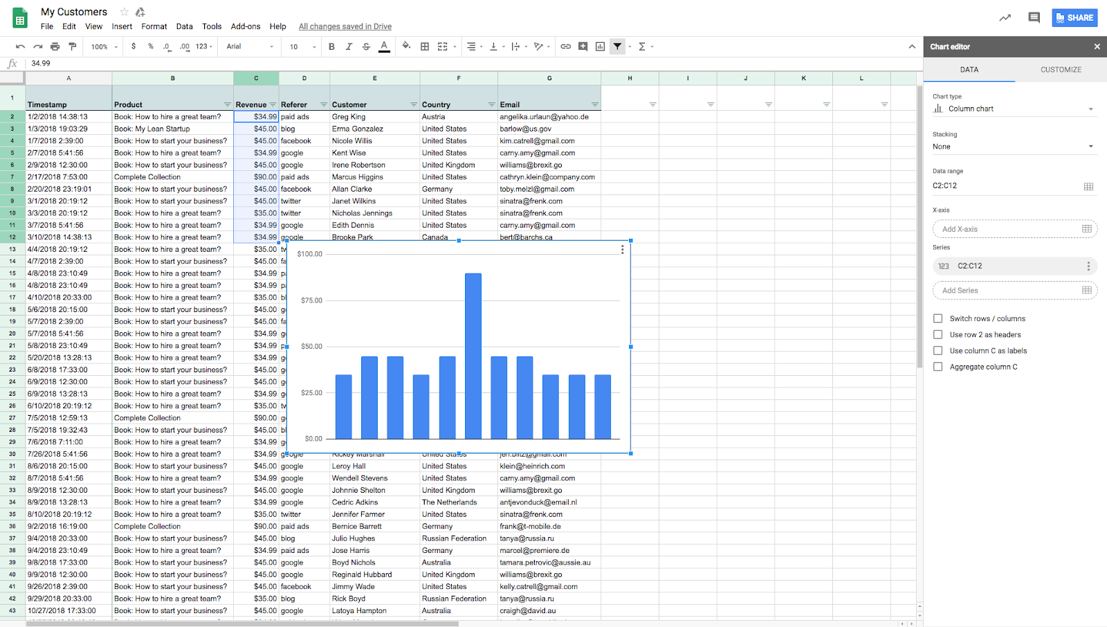
So, I'll highlight cells C2 through C12. Then, I'll click the chart icon in the toolbar along the top of the menu in Google Sheets.
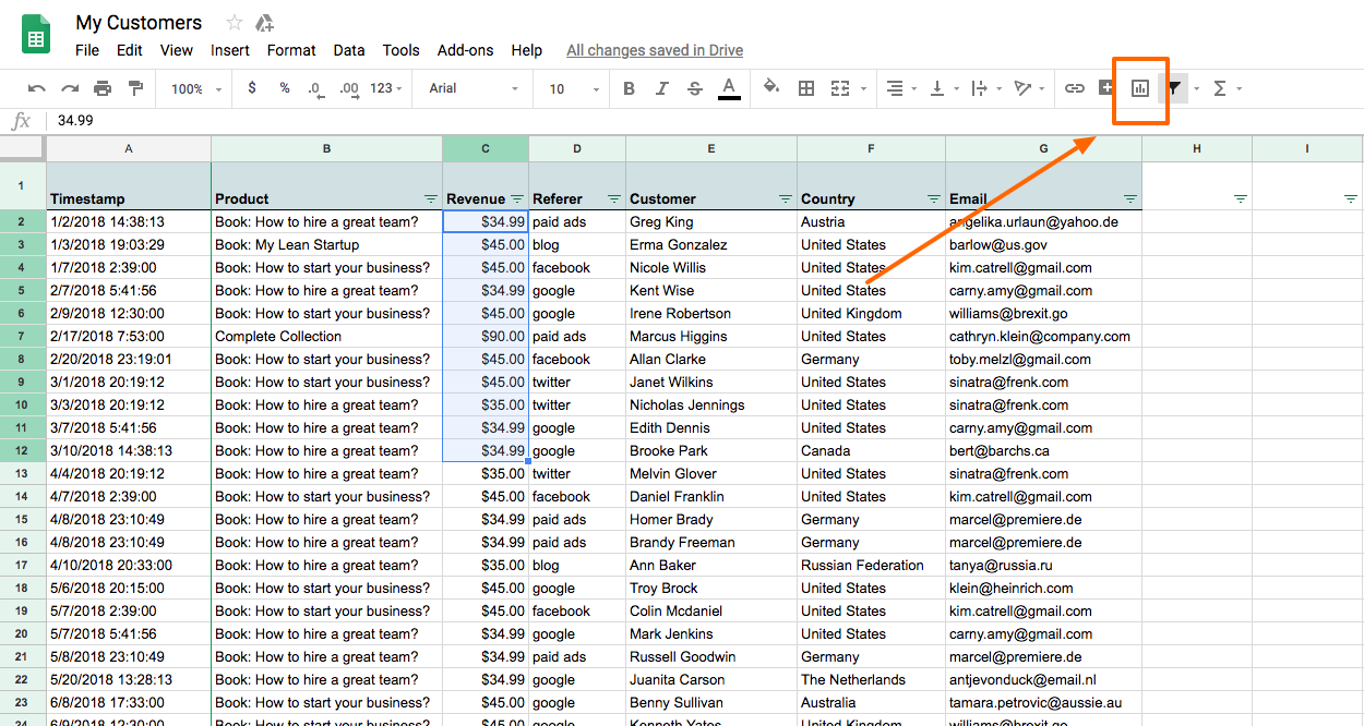
This will automatically display the data I've just highlighted in my spreadsheet in bar graph form.
How to Label a Bar Graph in Google Sheets
Now that you've created a bar graph in Google Sheets, you might want to edit or customizer the labels so that the data you're showing is clear to anyone who views it.
To add or customize labels in your bar graph in Google Sheets, click the 3 dots in the upper right of your bar graph and click "Edit chart."
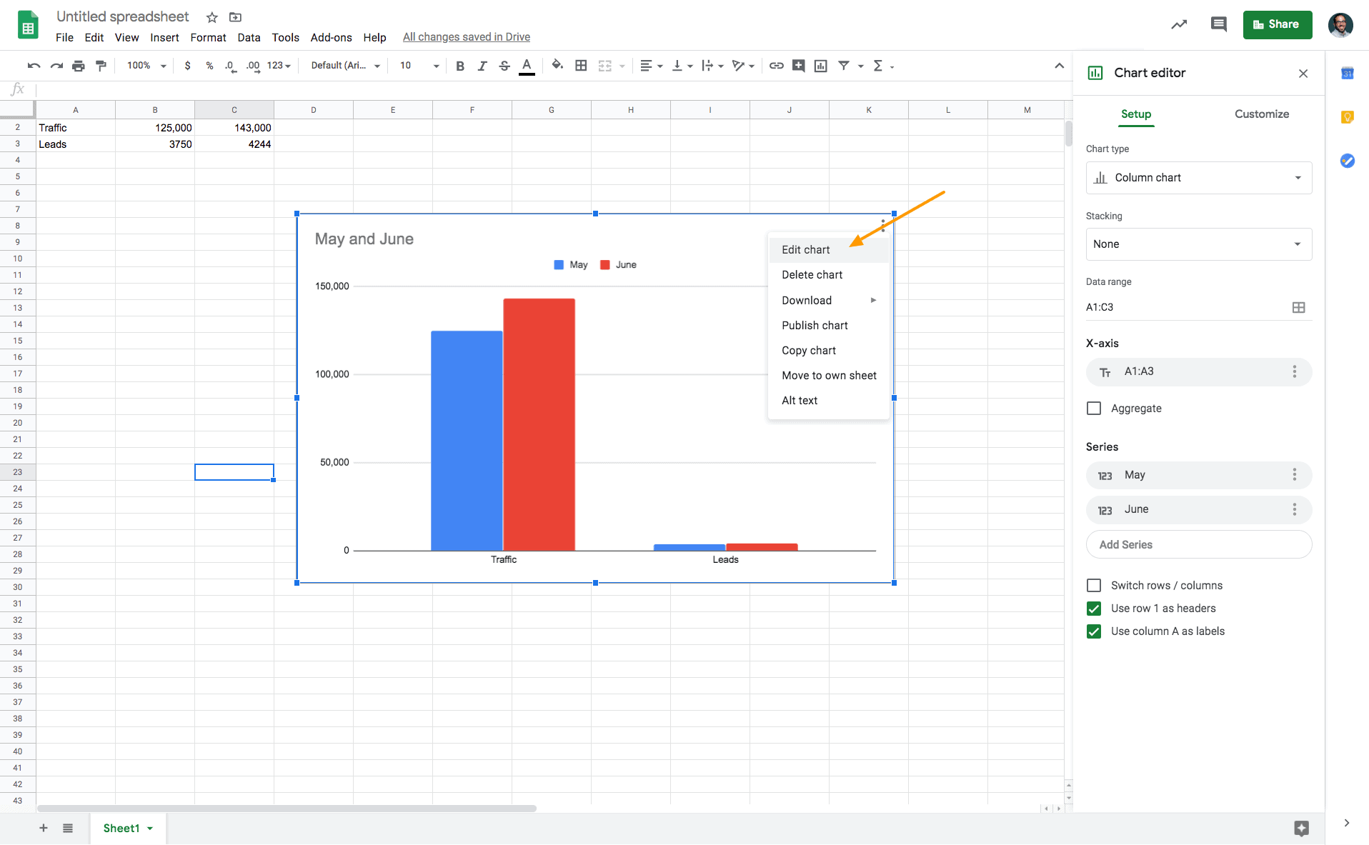
In the example chart above, I'd like to add a label that displays the total amount of website traffic and leads generated in May and June. To do so, I'll need to click each month under "Series", then "Add Labels", and then select the specific range from my spreadsheet that I'd like to display as a label.
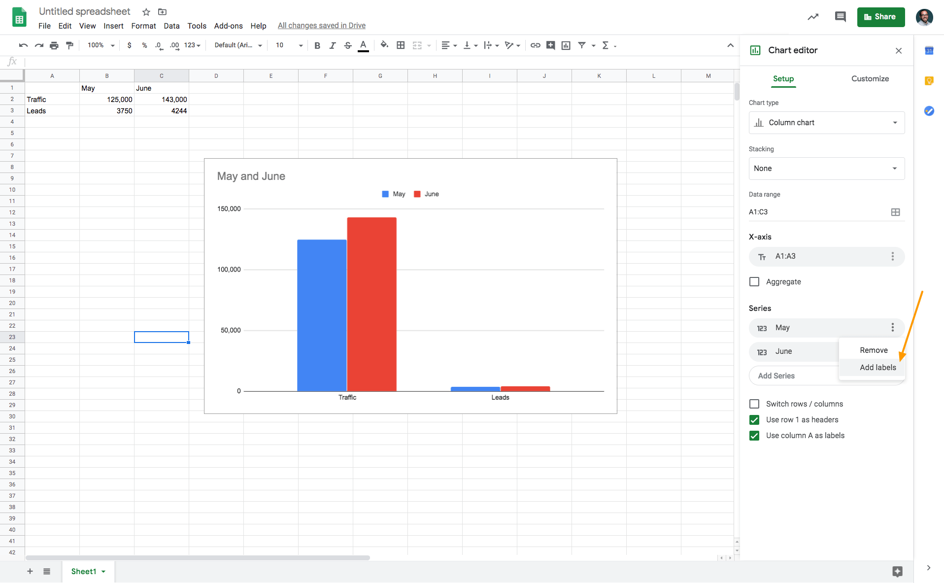
In this case, I'd select "May" and "June" in order to use the data from those columns as labels in my bar graph.
Next, I'll do the same thing for "June."
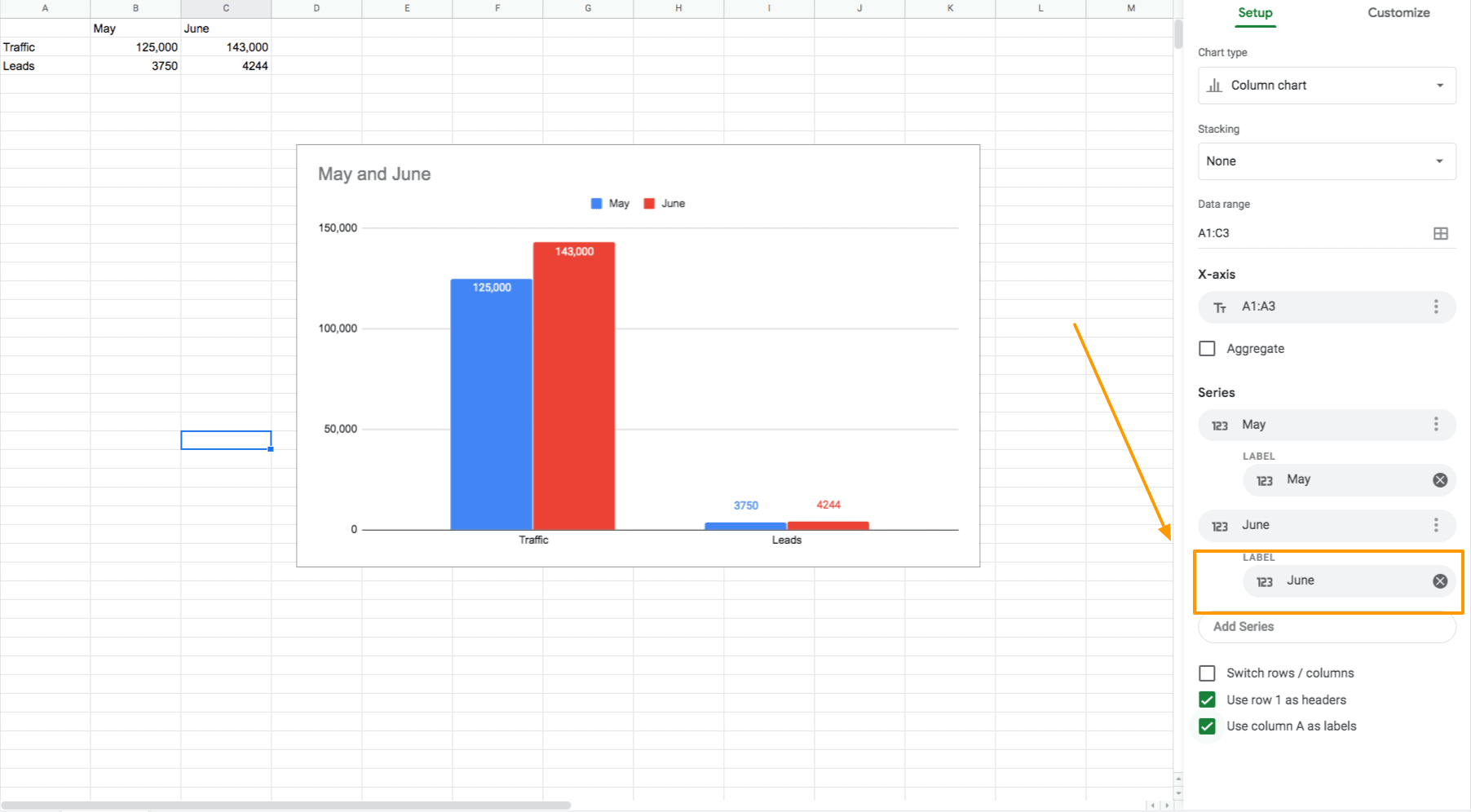
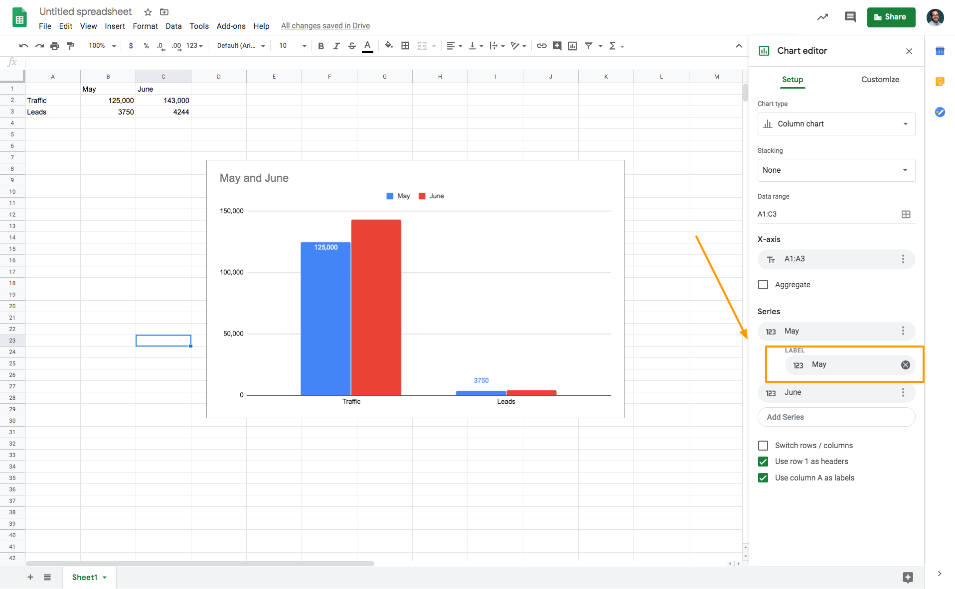
Now I've added labels showing the specific volume of traffic and leads generated in May and June.
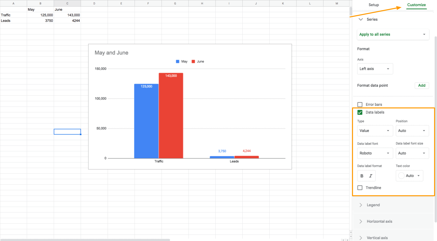
Next, if you'd like to customize the look of your labels––type, font, size, color, etc.––select "Customize" from the chart editor and you'll find all of your options.
How to Change a Visualization in Google Sheets
Want to change the bar graph visualization to something else?
On the chart editor on the right-hand side of your spreadsheet, click the "Chart Type" dropdown menu.
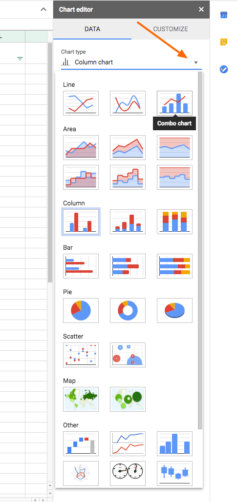
Here, you'll see all the different options for visualizing the data you've highlighted in your spreadsheet. Select the one you'd like and your data visualization will change within your spreadsheet automatically.
How to Add Error Bars in Google Sheets in 4 Steps
Error bars are used to visually illustrate expected discrepancies in your dataset.
In this example, I'm going to try to visualize data from my office supplies shopping list. So, to add error bars in Google Sheets, you'll need to follow these 4 steps…
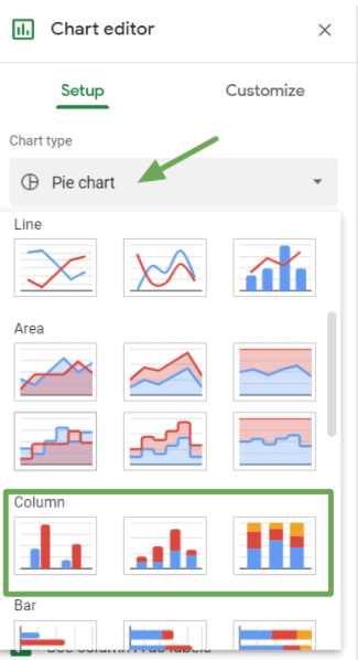
1. Highlight and insert the values you'd like to visualize
2. Google Sheets automatically visualizes your data as a pie chart. To change it, click on the chart type drop-down and then select column.
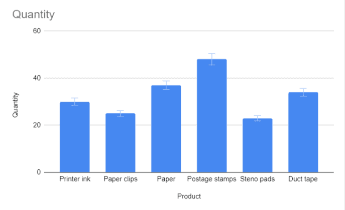
Here's what your chart should look like…

3. To add error bars to the above chart, still on the chart editor pane, navigate to customize and click on series
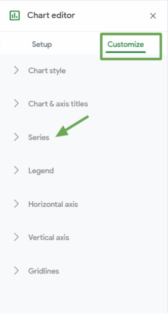
4. Select the error bars option..
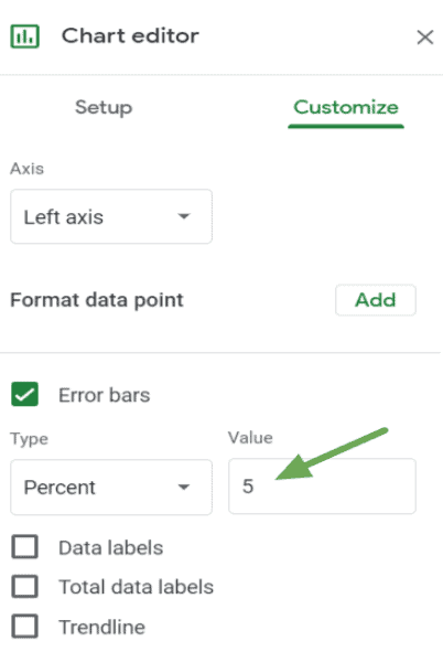
Depending on the expected difference in value(s), you may choose to increase or decrease the number, in my case I chose 5%.
Your percentage error bars should look like this…
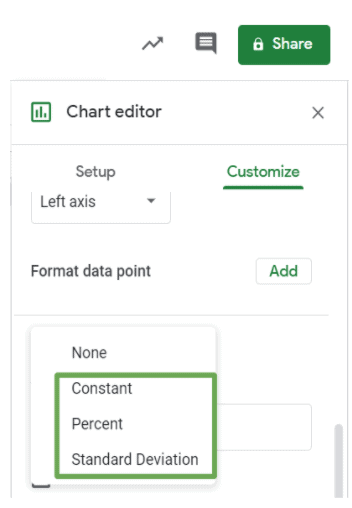
In addition, there are other types of error bars to choose from depending on how uncertain you are about your data.
How to Integrate Google Sheets with Databox
So what happens when you want to visualize data from multiple spreadsheets in one place?
For example, say you want to visualize top-of-funnel metrics like Sessions, but you also want to include downstream performance KPIs like signups and revenue, too?
In many cases, this data is pulled from different tools and is, therefore, located in several different Google Spreadsheets. This is when things get messy and complicated and make data visualization in a tool like Google Sheets impractical.
Here are a couple other reasons why Google Sheets isn't ideal for ongoing performance monitoring:
- You have to pull the data into the spreadsheet and manually keep it updated
- There isn't an easy way to share graphs without copying and pasting into slide decks (by the time you do, the data is outdated)
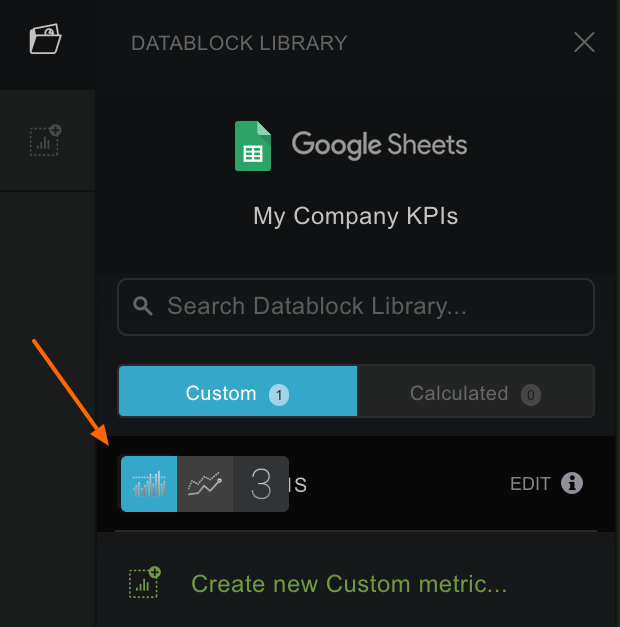
Now, with Databox's integration with Google Sheets, you can simply connect your Google spreadsheets to Databox and visualize any of the data you have stored in seconds.
Here's a quick video on how it works. (Skip ahead if you'd rather view the skimmable directions below.)
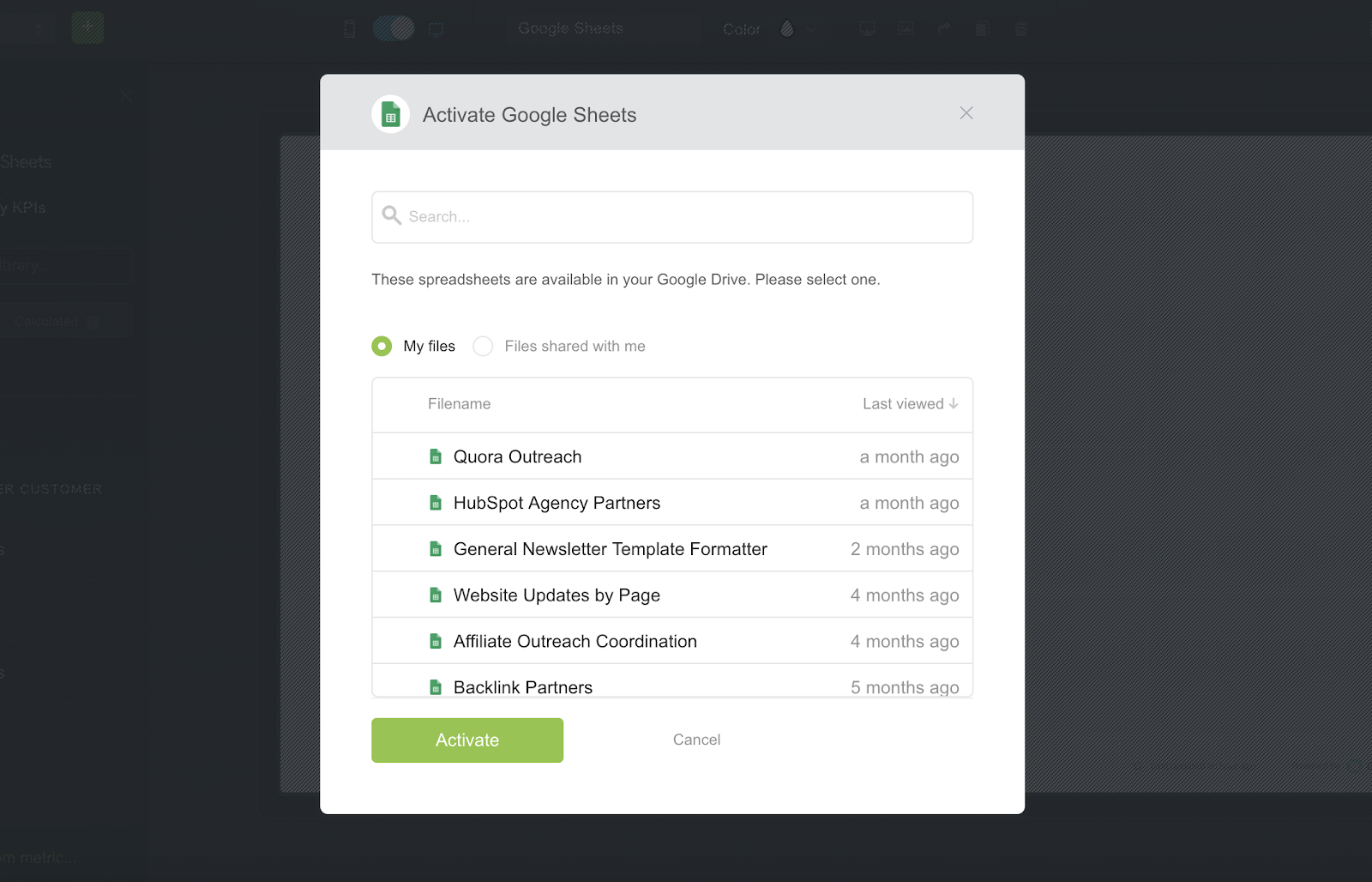
First, in the dashboard designer, you'll want to connect the spreadsheet you're looking to pull data from.
Then, you'll select the specific spreadsheet you'd like to pull data from.
Once you've selected the spreadsheet you want, you'll then create the specific metrics you're looking to visualize in the spreadsheet editor. This is super easy, as all you need to do is highlight the cells you're looking to pull data from.
First, you'll select the data range you'd like to pull data from. Here, I select the entire year of 2018 in row 1.
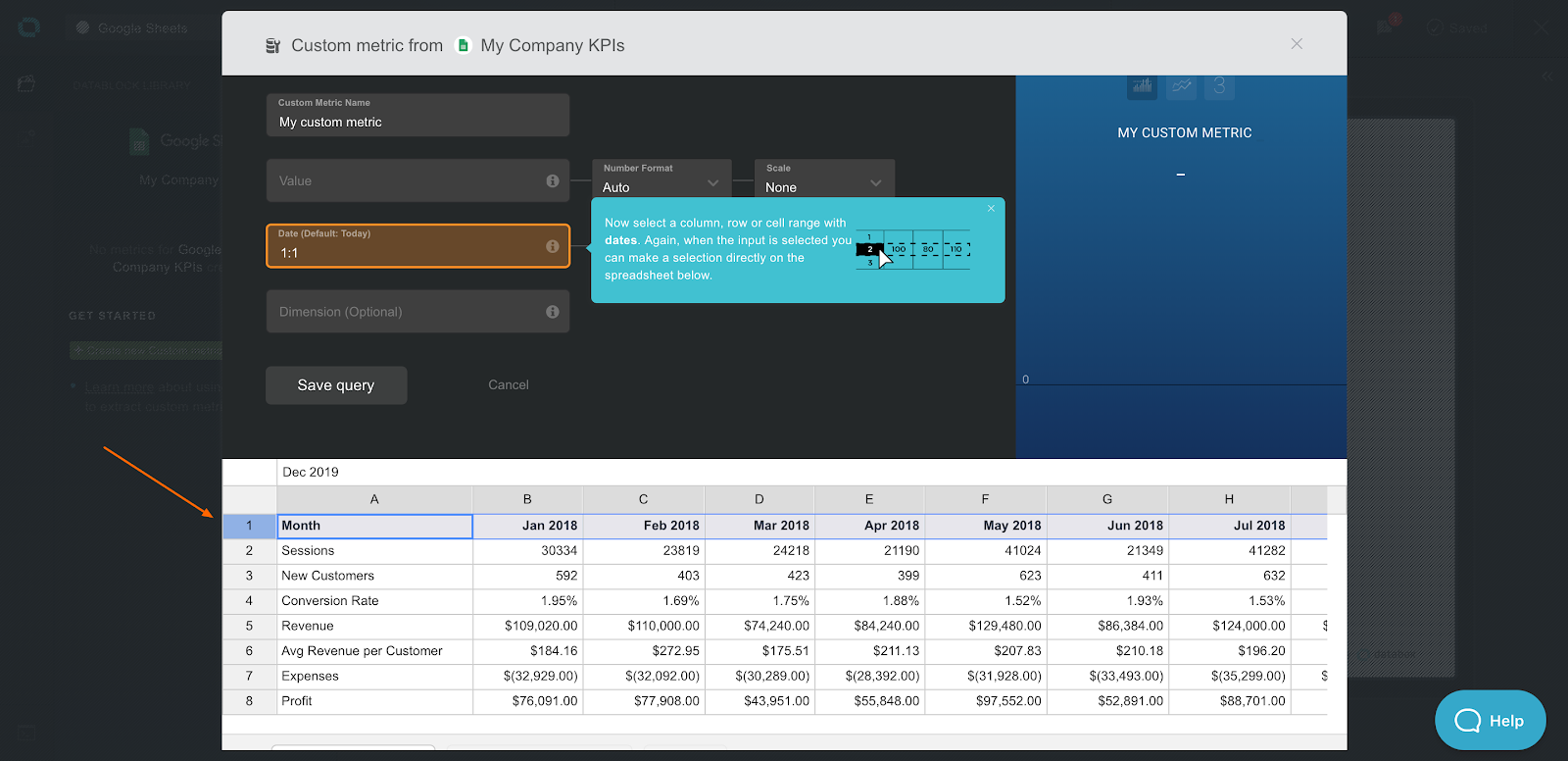
Next, you'll select the specific value you need to visualize by highlighting the specific rows or cells. In this case, I chose "Sessions."
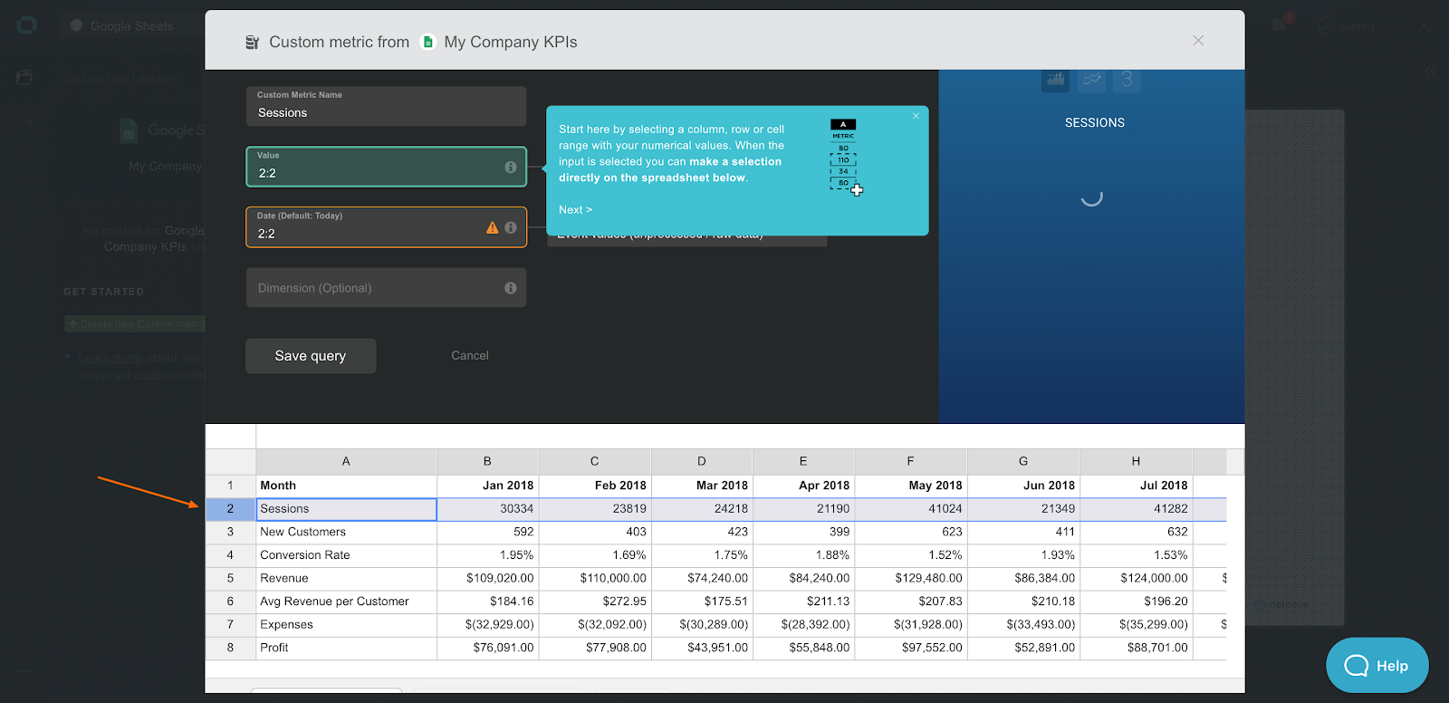
Throughout the process, you'll be able to see a preview of the data visualization you're building at the top right-hand side of the preview window. (Seen below.)
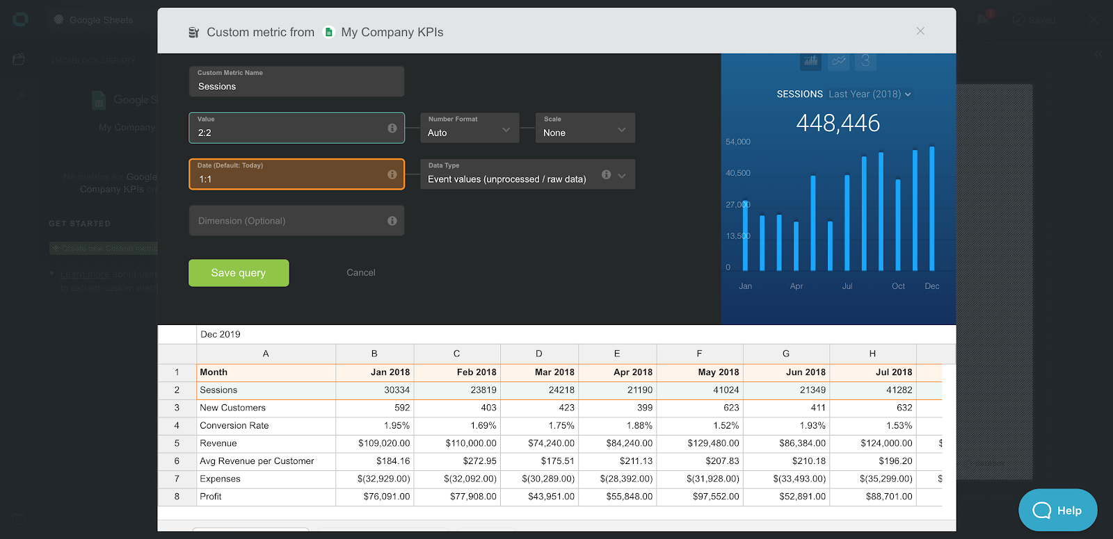
Once everything looks good, click 'Save' and your custom metric is now stored in Databox for you to add to any dashboard you'd like.
Want to change the visualization type? Changing the visualization for a specific metric is as easy as hovering over the metric listing on the left-hand menu. Here, you'll see hover options for the different visualization available for that metric.
Simply select the one you'd like and add it to your dashboard.
Connect Your Spreadsheets with Databox
The Google Sheets integration is available with all plans that include our Query Builder functionality. If your plan has access to Query Builder, you can log in and start using the Google Sheets integration, as of today.
If you are using a free, agency free or basic account, log in and request a trial of Query Builder.
Not using us at all? Start with a free account.
How to Draw Chart Bar Google Docs
Source: https://databox.com/how-to-create-a-bar-graph-in-google-sheets